Autoencoder using Python

What is an Autoencoder?

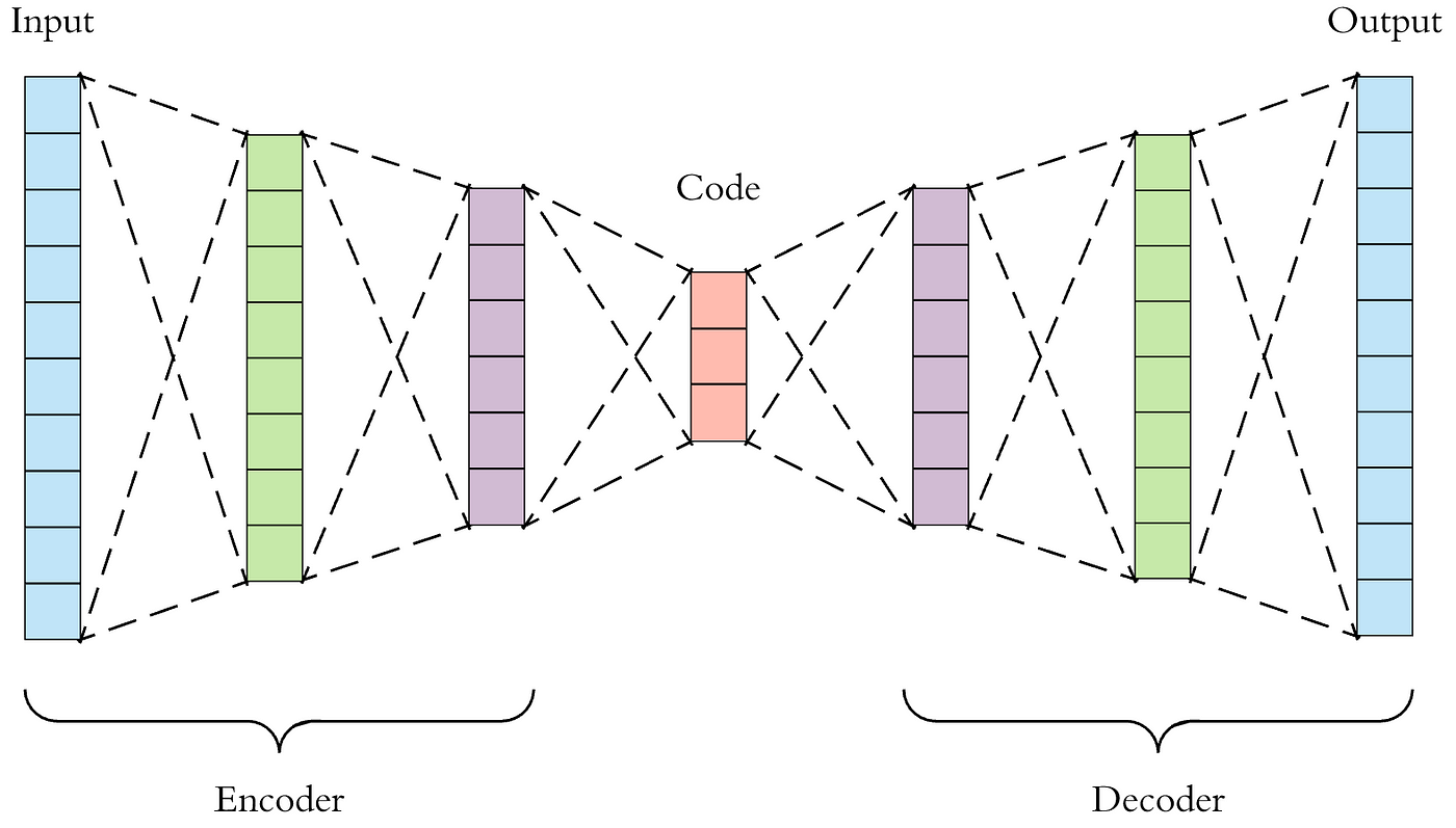
An Autoencoder is a type of artificial neural network used to learn efficient codings of data. The aim is to learn a representation (encoding) for a set of data, typically for the purpose of dimensionality reduction. The network consists of two main parts:

1. Encoder: This part compresses the input data into a latent-space representation (a smaller dimensional space).
2. Decoder: This part reconstructs the input data from the compressed latent-space representation.

Autoencoders are trained to minimize the difference between the input and output, which encourages the model to learn an efficient representation of the data. Because autoencoders are unsupervised, they don't require labeled data.

Anomaly Detection using Autoencoder

Anomaly detection involves identifying data points that don't fit the expected pattern. In the context of autoencoders, anomalies are identified based on the reconstruction error. If the reconstruction error (the difference between the input and the output) is higher than a certain threshold, the data point is considered an anomaly.

Python Code for Anomaly Detection using Autoencoder

Here’s how you can implement a simple autoencoder for anomaly detection:

import numpy as np
import pandas as pd
from tensorflow.keras.models import Model
from tensorflow.keras.layers import Input, Dense
from sklearn.preprocessing import MinMaxScaler
from sklearn.model_selection import train_test_split
from sklearn.metrics import mean_squared_error
import matplotlib.pyplot as plt

# Step 1: Generate synthetic data
data = np.random.normal(0, 1, (1000, 20))

# Introduce anomalies
anomalies = np.random.normal(0, 5, (50, 20))
data_with_anomalies = np.vstack([data, anomalies])

# Step 2: Normalize the data
scaler = MinMaxScaler()
data_scaled = scaler.fit_transform(data_with_anomalies)

# Step 3: Split the data into training and testing sets
X_train, X_test = train_test_split(data_scaled, test_size=0.2, random_state=42)

# Step 4: Build the Autoencoder Model
input_layer = Input(shape=(X_train.shape[1],))

# Encoder
encoded = Dense(16, activation='relu')(input_layer)
encoded = Dense(8, activation='relu')(encoded)
encoded = Dense(4, activation='relu')(encoded)

# Decoder
decoded = Dense(8, activation='relu')(encoded)
decoded = Dense(16, activation='relu')(decoded)
decoded = Dense(X_train.shape[1], activation='sigmoid')(decoded)

# Autoencoder Model
autoencoder = Model(inputs=input_layer, outputs=decoded)
autoencoder.compile(optimizer='adam', loss='mse')

# Step 5: Train the Autoencoder
history = autoencoder.fit(X_train, X_train,
                          epochs=50,
                          batch_size=32,
                          validation_split=0.1,
                          shuffle=True)

# Step 6: Predict and Evaluate Anomalies
X_test_pred = autoencoder.predict(X_test)

# Calculate the Mean Squared Error (MSE)
mse = mean_squared_error(X_test, X_test_pred, multioutput='raw_values')

# Define a threshold for anomaly detection
threshold = np.percentile(mse, 95)

# Identify anomalies
anomalies = mse > threshold
print(f"Number of anomalies detected: {np.sum(anomalies)}")

# Step 7: Visualize Results
plt.figure(figsize=(10, 5))

# Plot the loss over epochs
plt.subplot(1, 2, 1)
plt.plot(history.history['loss'], label='Training Loss')
plt.plot(history.history['val_loss'], label='Validation Loss')
plt.legend()
plt.title('Training and Validation Loss')

# Plot MSE histogram
plt.subplot(1, 2, 2)
plt.hist(mse, bins=50)
plt.axvline(threshold, color='red', linestyle='--')
plt.title('MSE Histogram with Threshold')

plt.show()
 

Explanation:

1. Data Generation: Synthetic data is generated with normal distribution. Some anomalies are introduced with higher variance.

2. Data Normalization: The data is normalized using MinMaxScaler.

3. Autoencoder Model: The autoencoder is built with a three-layer encoder and decoder. The model is compiled using the Adam optimizer and MSE loss.

4. Training: The autoencoder is trained to reconstruct the input data.

5. Anomaly Detection: After training, the model's reconstruction error is calculated for the test set. A threshold is set (95th percentile), and data points with higher errors are flagged as anomalies.

6. Visualization: Loss curves and MSE histogram are plotted to visualize the training process and the threshold for anomaly detection.

Types of mean in statistics

In statistics, several types of means are used to summarize data, each with its own significance and use cases. The most common types include:

1. Arithmetic Mean
2. Geometric Mean
3. Harmonic Mean
4. Weighted Mean
   

Let's explore each of these means and see how they can be computed using Python.

1. Arithmetic Mean

The arithmetic mean is the most common type of mean, often referred to simply as the "average." It is calculated by summing all the values and dividing by the number of values.

Formula:

$$\text{Arithmetic Mean} = \frac{\sum_{i=1}^{n} x_i}{n}$$

Python Example:

import numpy as np

data = [10, 20, 30, 40, 50]
arithmetic_mean = np.mean(data)
print(f"Arithmetic Mean: {arithmetic_mean}")
 

2. Geometric Mean

The geometric mean is useful when dealing with data that involves multiplication or percentages, such as growth rates. It is calculated by multiplying all the values together and then taking the nth root, where n is the number of values.

Formula:

$$\text{Geometric Mean} = \left( \prod_{i=1}^{n} x_i \right)^{\frac{1}{n}}$$

Python Example:

from scipy.stats import gmean

data = [10, 20, 30, 40, 50]
geometric_mean = gmean(data)
print(f"Geometric Mean: {geometric_mean}")
 

3. Harmonic Mean

The harmonic mean is useful when dealing with rates or ratios, such as speed or density. It is calculated as the reciprocal of the arithmetic mean of the reciprocals of the data values.

Formula:

$$\text{Harmonic Mean} = \frac{n}{\sum_{i=1}^{n} \frac{1}{x_i}}$$

Python Example:

from scipy.stats import hmean

data = [10, 20, 30, 40, 50]
harmonic_mean = hmean(data)
print(f"Harmonic Mean: {harmonic_mean}")
 

4. Weighted Mean

The weighted mean is an average that takes into account the relative importance (weight) of each value. It is useful when different data points contribute differently to the overall mean.

Formula:

$$\text{Weighted Mean} = \frac{\sum_{i=1}^{n} w_i \cdot x_i}{\sum_{i=1}^{n} w_i}$$

Where $w_i$ is the weight for each value $x_i$.

Python Example:

data = [10, 20, 30, 40, 50]
weights = [1, 2, 3, 4, 5]  # Weights corresponding to each data point
weighted_mean = np.average(data, weights=weights)
print(f"Weighted Mean: {weighted_mean}")
 

Summary of Outputs:

• Arithmetic Mean: $30.0$
• Geometric Mean: Approximately $26.379$
• Harmonic Mean: Approximately $21.818$
• Weighted Mean: $40.0$

Explanation:

• Arithmetic Mean is a simple average and is widely used for data where each observation is equally important.
• Geometric Mean is more appropriate for data that involves products, such as growth rates.
• Harmonic Mean is particularly useful for average rates, such as speed or density.
• Weighted Mean adjusts the mean by giving different importance to different data points, useful in scenarios where some data points have more significance than others.

What is Axiomatic probability?

Axiomatic probability is a formal approach to probability theory that is based on a set of axioms or rules. These axioms, introduced by the Russian mathematician Andrey Kolmogorov in 1933, form the foundation of modern probability theory. 

The three main axioms are:

1. Non-negativity: For any event $A$, the probability of $A$ is a non-negative number.

   $$P(A) \geq 0$$

2. Normalization: The probability of the entire sample space $S$ is 1.

   $$P(S) = 1$$

3. Additivity: For any two mutually exclusive (disjoint) events $A$ and $B$, the probability of their union is equal to the sum of their probabilities.

   $$P(A \cup B) = P(A) + P(B) \quad \text{if } A \cap B = \emptyset$$

Python Example:

Let's implement a simple example in Python to demonstrate these axioms.

# Define the sample space
S = {"H", "T"}  # Let's say we have a simple coin toss scenario: Heads (H) or Tails (T)

# Define a probability function that satisfies the axioms
def probability(event):
    event_space = {"H": 0.5, "T": 0.5}  # Assign probabilities to each outcome
    return sum(event_space[e] for e in event)

# Axiom 1: Non-negativity
A = {"H"}
print(f"P(A): {probability(A)} >= 0")  # Output should be non-negative

# Axiom 2: Normalization
B = {"H", "T"}
print(f"P(S): {probability(B)} == 1")  # The probability of the entire sample space should be 1

# Axiom 3: Additivity
C = {"H"}
D = {"T"}
print(f"P(C ∪ D): {probability(C.union(D))} == P(C) + P(D): {probability(C) + probability(D)}")
# The sum of P(C) and P(D) should equal P(C ∪ D) because C and D are disjoint (mutually exclusive)
 

Explanation:

• Non-negativity: The probability of event $A$ (e.g., getting a Head) is defined as 0.5, which is non-negative.

• Normalization: The probability of the entire sample space $S$ (e.g., either getting a Head or a Tail) is calculated as 1, satisfying the normalization axiom.

• Additivity: Since getting a Head (C) and getting a Tail (D) are mutually exclusive events, the probability of getting either a Head or a Tail (C ∪ D) is the sum of their individual probabilities.

  Output:

  Running the above code will produce:

  P(A): 0.5 >= 0
  P(S): 1 == 1
  P(C ∪ D): 1.0 == P(C) + P(D): 1.0
  

Architecture of 80386

The internal architecture of 80386DX is divided into following sections:

• Central processing unit
  • Execution unit
  • Instruction decode unit
• Memory management unit
  • Segmentation unit
  • Paging unit
• Bus control unit

The central processing unit is further divided into execution unit and instruction unit. The memory management unit consists of a segmentation unit and a paging unit . These unit operate in parallel. Fetching, decoding, memory management and bus access for several instruction are performed simultaneously. This parallel operation is called pipelined instruction processing .

Execution unit : The execution unit read the instruction from the instruction queue and executes the instructions. It consists of three subunit: control unit, data unit and protection test unit .

1. Control unit : It contains microcode and special hardware. The microcode and special hardware allow 80386DX to reduce time required for execution of multiply and divide instruction . It also speeds up the effective address calculation .
2. Data unit : The data unit contain the ALU, eight 32-bit general perpose registers and a 64-bit barrel shifter. The barrel shifter is used for multiple bit shifts in one clock. Thus it increases the speed of all shift and rotate operation. The multiply/divide logic implement the bit shift rotate algorithm to complete the operation in minimum time. The entire data unit is responsible for data operation requested by the control unit .
3. Protection test unit : the protection test unit check for segmentation violations under the control of the microcode.

Instruction decode unit : The instruction decode unit takes the instruction bytes fron the code prefetch queue and translates them into microcode the decoded. The decoded instruction are then stored in the instruction queue. They are passed to control section for deriving the necessary control signals .

Segmentation unit : The segmentation unit translates logic addresses into linear addresses at request of the execution unit . The segmentation unit compares the effective address for the length limit specified in the segment descriptor. The segment unit adds the segment base and the effective address to generate linear address. Before calculation of linear address it also check for access rights. It provides a 4-level protection mechanism for protecting and isolating the system code and data from those of the application program.

Paging unit : When the 80386DX paging mechanism is unabled, the paging unit translates linear addresses generated by the segmentation unit or the code prefetch unit into physical addresses. If paging unit is not enabled, the physical address is the same as the linear address, and no translation is necessary. The paging unit gives physical address to the bus interface unit to perform memory and I/O accesses . It organizes the physical memory in term of pages of 4 kbytes size each .

The control and attribute PLA check the privileges at the page level. Each of the page maintain the paging information of the task. The limit and attribute PLA checks segment limits and attributes at the segment level to avoid anvalid accesses to code and data in the memory segments .

Bus control unit : The bus control unit is the 80386DX's communication with the out side world. It provide a full 32-bit bi-directional data bus and 32-bit address bus. The bus control unit is responsible for the following operations :

1. It accepts internal request for code fetch and data transfer from the code fetch unit and from the execution unit. It then prioritize the request with the help of prioritize and generate signal to perform bus cycles.
2. It sends address, data and control signal to communicate with memory and I/O devices. The address driver drives the bus enable and address signal A0-A31 and the transceiver interface the internal data bus with the system bus .
3. It control the interface to the external bus masters and coprocessors.
4. It also provides the address relocation facility.

Instruction prefetch unit : The instrction prefetch unit fetch sequentially the instruction byte stream from the memory. It uses bus control unit to fetch instruction bytes when the bus control unit is not performing bus cycle to execute an instruction. These prefetched instruction bytes are stored in the 16-byte code queue. A 16-byte code queue holds these instruction until the decoder needs them the prefetcher always fetches instruction in the order in which they appear in the memory. It fact, the prefetcher simply reads code one double word at the time, not caring whether it's bringing in complete instruction are executed, the contents of the prefetched and decode queues are cleared out. In this case, prefetcher again starts filling its queue.

Instruction predecode unit : The instruction predecode unit takes instruction bytes from the instuction prefecth queue an translate them into microcode the decoded instruction are then stored in instruction queue.

References:

1. Wikipedia page on 80386.
2. “Advanced 80386 Programming Techniques” by James L. Turley, TMH Publications.
3. http://nptel.ac.in
4. http://nptel.iitk.ac.in
5. http://www.delorie.com
6. http://homes.ieu.edu.tr

What is 10,13 in Assembly Language variable declaration?

In many assembly language programs written for x86 architecture, the values 10, 13 are written in data segment declaration.

e.g.

    .data

     message db 10, 13, 'abcd$'

Here the string will be declared and it will have the values declared in front of it. The actual array will be,

message:

0AH

0DH

41H

42H

43H

44H

24H

10         13         'a'          'b'         'c'         'd'         '$'

The respective ASCII characters of these values will be printed till '$'. It is considered as end of the string character. 'a' 'b' 'c' 'd' are printable characters but 10 & 13 are non-printable characters .

In short,they are control characters chart below.(Reference -Wikipedia).

10 is called as LF or Line Feed or new line and 13 is called as CR or Carriage return.

These character are used to control the cursor position. The 10 shifts cursor on new line with same column no. and 13 returns the cursor to its initial position of line that is at start of the line!

So, every time you make use of these control characters as the part of string or any array. It shifts the cursor to new line and at the start of the line.

(Note – the term carriage return (CR) is taken from printer's operation. When printer finishes one line printing, it shifts to new line but it prints head moves to start of new line).

LF & CR are equivalent to \n & \r used is print statement of high level programming languages.

Lets take an Example.

Declare variable as

   .data

      message db 10,13,'Welcome$'

and print using,

    MOV AH, 09H

  LEA DX, MESSAGE

  INT 21H

Now make some changes in declaration as,

   .data

   message db 10, 13, 'Wel', 10, 13, 'come$'

Check the output by printing this message.

Batch file for execution of multiple commands

There are only three kinds of file in DOS which are directly executable. These are .exe, .com,and .bat. Out of these, .exe and .com are executable files. The .bat is batch file or a scripting file.

Whenever we want to execute multiple commands at a time, we may use the batch file. We just need to add all commands in a file whose extension is .bat. This is very usefull while executing a assembly language program.

For example, you have written a program named myprog.asm and you want to assemble, link and execute in one command. Then just create a file called run .bat and type in it.

   masm myprog.asm;

   link myprog;

   myprog

This file must be present in your current working directory. i.e /masm. Now, after typing 'run' (name of batch file ) on terminal all above commands will get executed.

See the screenshots below:

Final execution:

How to set video mode in X86 assembly?

The interrupt no. 10H is dedicated for all kinds on video operation of 8086/8088 DOS system. The function number 01 with interrupt 10H is used to set the video mode.

The mode values must be set in AL register.

The values 00h to 03H specifies the text modes of DOS. Remaining are Graphics modes. The default text mode is 80 X 25. That is, 80 character per line X 25 line per screen page.

So, this text resolution can be changed with the help of interrupt no. 10H.

By setting any video mode, the display screen will be cleared automatically.

For e.g.

    MOV AH,00H

  MOV AL,00H

  INT 10H

This will set the video mode (text) of 40 characters per line X 25 line per page. It changes the default resolution. Likewise, we may use different kind of values in AL register.

These are:

00H – 40 X 25 (text) color burst OFF

01H – 40 X 25 (text)

02H – 80 X 25 (text) color burst OFF

03H – 80 X 25

04H – 320 X 200 pixels (graphics)

05H – 320 X 200 pixels (graphics) color burst OFF

06H – 640 X 200 (graphics)

... and so on.

To Know more about these values, refer book “Advanced MS-DOS Programming” by Ray Duncan (BPB Publications).